Challenges of Prolonged Follow-up and Temporal Imbalance in Pragmatic Trials: Analysis of the ENCOURAGE Trial

Plans

Enrollment and baseline data collection occurred between February and August 2010, with communities randomized using permuted blocks. The typical 2.5- hour one-way travel time to the partner communities required that we enroll 1 community at a time, with some communities requiring more than 1 date.

Reality

The original recruitment schedule had to be modified several times due to unexpected events (eg, funerals) in our partner communities, resulting in temporal imbalance in the enrollment of intervention and control participants (Figure 1, Panel A). Specifically, participants enrolled in February, July, and August were primarily in the control group while most enrollment in April, May and June was in the control group.

• Download figure
• Open in new tab
• Download powerpoint

• Download figure
• Open in new tab
• Download powerpoint

Figure 1

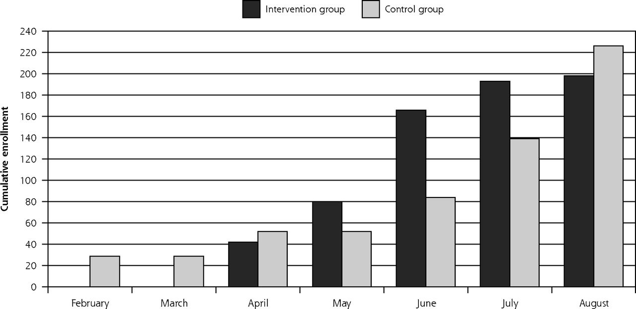
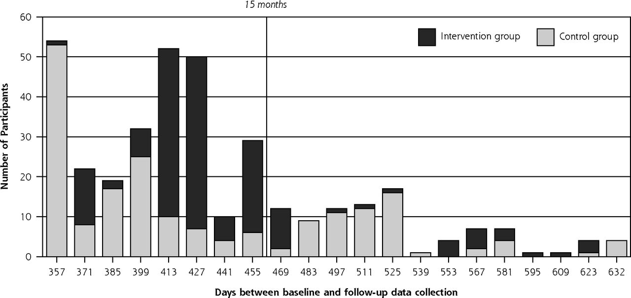
The timing of baseline and follow-up data collection in the ENCOURAGE trial displaying temporal differences by study group.

B. Elapsed time from baseline data collection to follow-up in days, with a vertical line at 15 months, the standard cut-off point for 1-year follow-up. By the 15-month point, 268 participants had been followed up, of whom 51.4% (138) were in the intervention group and 48.5% (130) in the control group. After that point, 92 participants were followed up, of whom 32.6% (30) were in the intervention group and 67.4% (62) were in the control group.

Analytic Challenges Created

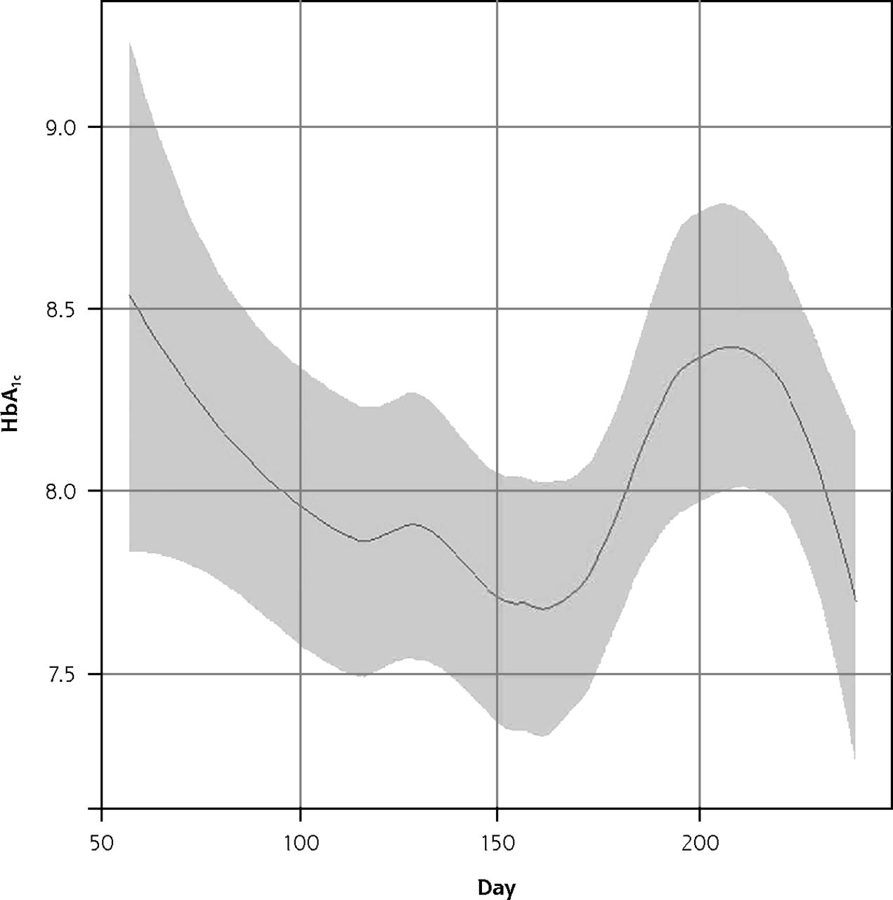
Figure 2 shows the seasonal variation in baseline HbA_1c in ENCOURAGE. The imbalance in enrollment times between groups created the possibility of confounding seasonal trends and study group characteristics.

• Download figure
• Open in new tab
• Download powerpoint

Figure 2

The seasonal trend in HbA_1c levels in the ENCOURAGE trial.

Note: The figure reflects all baseline observations reported in calendar days where January 1 is day 1 and December 31 is day 365. The period represented runs from late February to late August.

Implications

This kind of temporal imbalance at baseline can easily occur if recruitment and randomization occur in clusters, especially if logistic constraints require them to occur sequentially over a period of time-spanning seasons.

Plans

We planned to follow up on participants in both groups between June 2011 and January 2012, approximately 1 year after baseline, by community, in the same order as recruitment, allowing up to 3 months deviation from this schedule.

Reality

The actual course is displayed in Figure 1, Panel B. Only 268 participants (63%) had follow-up data collection within 15 months of enrollment. Although there was no significant imbalance between study groups in the proportions who had follow-up within 15 months, most of the first 50 participants followed up were in the control group.

To maximize the reach and generalizability of this pragmatic trial, we offered in-home visits for data collection, and we eventually achieved 85% retention by prolonging the follow-up period. Among participants completing follow-up more than 15 months after baseline, 62 (67%) were control and 30 (33%) were intervention participants, a considerable imbalance.

While we collected follow-up data from June 2011 to February 2012, the time elapsed from baseline to follow-up for individuals ranged from 10.3 to 20.8 months. Although there was no statistical difference in mean days to follow-up (Control 426, Intervention 436; t-test P = .12) there was a significant difference in distributions (Wilcoxon P <.001).

Analytic Challenges Created

Any observed effect of the intervention may have changed over time; for instance, if the peak intervention effect occurred at or before 15 months and diminished thereafter, we would expect to observe a smaller effect among participants whose follow-up data collection was much beyond 15 months. The usual approach to analyzing trial data would not reflect these temporal nuances.

Implications

The lesson for similar trials is that there can be a trade-off between adhering to protocol despite a low follow-up on one hand, and breaking protocol to achieve more comprehensive follow-up with a more representative cohort on the other. The former allows for a standard analysis, while the latter requires a more complicated analysis to account for variable times to follow-up. A low follow-up (like the 63% we managed within 15 months) may bias the results of the trial, while a lengthier follow-up period may allow not just more complete follow-up, but also the possibility of tracking of changes in intervention effect over time.

Plans

The standard analytical approach for randomized trials relies on randomization to make control and intervention study participants comparable, with a balanced time from baseline to follow-up and variability small enough to render seasonal and secular trends unimportant. The overall effectiveness of the study is estimated as a distribution-appropriate difference between groups—for example, a difference in means, change, proportion experiencing an event, or survival time. Statistical significance is tested using an unadjusted test for a difference between groups. If there are statistically significant differences between groups at baseline, the main test may take the form of regression analysis with adjustment for unbalanced characteristics. Group randomized trials typically account for clustering by using regression with generalized estimating equations or mixed effects models. Furthermore, when the primary outcomes are change in baseline characteristics such as BMI or HbA_1c, it is also appropriate to adjust for the individual’s baseline value to control for regression to the mean.

Reality

We observed statistically significant baseline imbalances between groups in race (P <.001) and education (P = .05) with some indication of imbalance in income (P = .10). We therefore used regression models controlling for these factors and the baseline value for each outcome. For instance, our initial proposed model for change in BMI was this:

(1)

To account for the challenges discussed above, we augmented this model in a stepwise fashion. First, we added a term for elapsed study time at follow-up and an interaction term allowing the groups’ changes to differ over time. The new model for change in BMI was:

(2)

In this model the test for an intervention effect would be the significance of the group-by-time interaction term (β₇ ≠ 0). An advantage of this approach is that it explicitly makes use of the information on variable exposure to the intervention. The disadvantage is that it does not estimate a single intervention effect, but rather, indicates that the difference between the groups changed significantly over time.

The standard analysis can report results such as, “We observed a decrease in mean HbA_1c of xx at 1 year in the intervention compared with the control group (P = .0x).” In contrast, inclusion of a group-by-time interaction changes the interpretation to “we observed that the difference in mean HbA_1c between intervention and control groups changed significantly over time from 1 year to 2 years (P = .0x)” The latter can’t answer the question “how big was the intervention effect?” because the observed intervention effect changed over time. While this approach is valid and actually provides more information than estimating the difference at a single point in time, it is more difficult to comprehend and explain. For example, if an intervention group did worse initially but better later on, there may be no overall effect, but analysis with a group-by-time interaction might correctly identify that the differences between groups changed over time.

Second, we noted secular trends. For instance, both groups experienced an increase in LDL cholesterol, leading us to add another variable reflecting calendar time throughout the study as days from January 1, 2010. To account for seasonal variations in biometric measures, we added variables controlling for the season of baseline and follow-up data collection, defined in three-month intervals as Winter (January–March), Spring (April–June), Summer (July–September), and Fall (October–December).

The final linear model was operationalized as:

(3)

Initial results included negative estimates for the group-by-time interactions, meaning intervention effects were decreasing over time. As an intervention takes effect, we would expect the groups to diverge, with more improvement among the intervention group, but after the intervention ends or maximum effectiveness is reached, we would expect the intervention effect to plateau or decay. The ENCOURAGE intervention was planned to last 1 year, and given that follow-up extended well beyond 1 year after baseline, we surmised that follow-up observations might have spanned both the periods of increasing effect and decay, meaning that a linear fit would be inadequate.

There are several approaches to address nonlinear trends in data. One is to add higher powers of Time to the model (eg, Time² or Time³), essentially modeling the time trend as a polynomial function. While this is fairly intuitive, and polynomials readily capture effects that both rise and fall, polynomials often introduce artifacts toward the margins of the distribution (early or late follow-up times) because the higher powers dominate.³ Another approach would be to incorporate other transformations, such as log(Time). While sometimes useful, this is less intuitive and has the potential issue that because it only increases with time, it can be less useful for modeling an effect that rises and falls. Using regression splines is a strategy that retains the advantages of polynomials while limiting the disadvantages. In essence, splines model separate sections of the data using polynomials (eg, 0 to 150 days and 150 to 300 days) but with mathematical constraints that force them to join together smoothly. Further constraints are used at the margins to reduce distortions. The points defining the intervals for separate spline fits are called ‘knots’ (the knots in the above example would be at 0, 150 and 300 days) and the most commonly used splines are cubic. One potential disadvantage of splines is that they add another layer of complexity and often require the user to specify the order of the splines and the location of the knots.

To model our temporal trends, we used generalized additive mixed models (GAMM) to consider the potentially nonlinear changing pattern of the intervention effect over time.^3,4 The fitting process iteratively optimizes the model’s performance. The model is fit leaving some observations out and then validated using the excluded observations to quantify model performance. This method provides a good fit to the data without forcing the model to be linear, while penalized smoothing effectively guards against over-fitting. In our case the algorithm used splines to capture the nonlinearity, but the location and number of knots was determined iteratively by the algorithm rather than chosen explicitly. As with linear models using a group-by-time interaction, nonlinear models will not provide a single estimate of the intervention effect. Rather, they test for whether the control and intervention groups differ over time. A potential advantage is that by faithfully modeling changes over time, we could isolate any increasing intervention effect followed by plateau or decay.

When constructing the final model for each outcome, the overall time trend was fit as a linear term and the intervention effect (difference between groups) over time was allowed to be nonlinear. Initial models allowed the overall time trends to be nonlinear, but model fits provided no evidence suggesting that nonlinearity was required. The final model was similar to model (3) replacing the group-by-time terms with the penalized spline term for the intervention effect. We used an implementation of GAMM models by the package mgcv in the statistical programming language R, version 3.01, which allowed us to include community clusters as random effects.^4–6 Modeling was repeated, including the additional clustering of intervention participants within peer-advisors as well as communities, but results were not substantially different.

The results of the group-by-time models and the final GAMM fits for changes in BMI are shown in Figure 3. The heavy dashed line shows the group-by-time linear model. The heavy solid line, in contrast, shows the statistically significant nonlinear fit of the intervention effect over time with estimated degrees of freedom (EDF) of 5 indicating the importance of the nonlinearity. Examination of the plot shows how the estimated intervention effect changed over time. Intervention group participants followed up earlier and later than 15 months experienced greater weight loss than control participants followed at the same times, but those followed around 15 months may have had slight weight gain compared with control participants. From this observation it follows that the planned time of tightly scheduled follow-up could determine whether the intervention effect was judged to be positive, negative, or non-existent.

• Download figure
• Open in new tab
• Download powerpoint

Figure 3

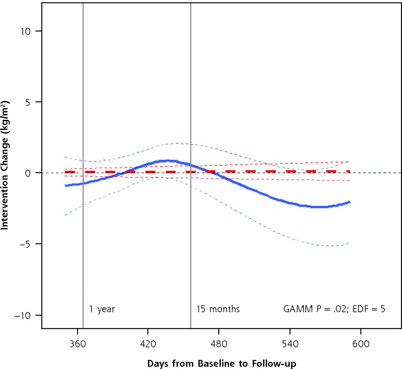
The change in BMI attributable to the intervention over time, by linear model and GAMM.

Note: The plot shows the adjusted model results for the difference between intervention and control groups (the intervention effect) with 95% confidence regions bounded by thin dashed lines. The heavy dashed line shows no linear effect over time, while the heavy solid line shows the GAMM results, which allow the effect over time to be nonlinear. The GAMM P <.05 and the estimated degrees of freedom (EDF) >1 indicate that the association is significant and that the nonlinearity is important.

GAMM = generalized additive mixed models.

Implications

The presence of temporal imbalance requires a thoughtful look at the data to consider which imbalances may require careful examination. In the case of the ENCOURAGE trial, considering all the factors seemed to be necessary; but any given trial may or may not have evidence for secular trends, seasonal trends, or nonlinear temporal trends in intervention effect. Ultimately, we all hope to have our studies go according to plan. In the event that they do not, these approaches show a way to uncover useful information even when a simple estimate of the trial’s effect is not feasible.